Note
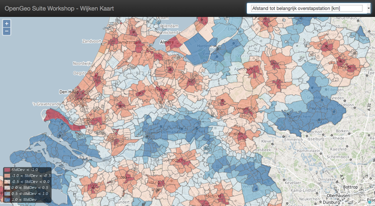
Check out the full demonstration application and play!
For this adventure in map building, we use the following tools, which if you are following along you will want to install now:
The basic structure of the application will be
This application exercises all the tiers of OpenGeo Suite!
In order to keep things simple, we will use a geographic unit that is large enough to be visible on a country-wide map, but small enough to provide a granular view of the data: a district (or wijk in Dutch). There are about 3000 districts in The Netherlands, enough to provide a detailed view at the national level, but not so many to slow down our mapping engine.
For this workshop we will be using the dataset Wijk- en Buurtkaart 2013. Which is a dataset that contains all the geometries of all municipalities, districts and neighbourhoods in the Netherlands, and its attributes are a number of statistical key figures.
Note
The next steps will involve some database work.
- If you haven’t already installed the OpenGeo Suite, follow the Suite installation instructions.
- Open up pgAdmin3 and create a spatial database named opengeo to load data into.
Loading the wijk_2013_v1.shp file is pretty easy, either using the command line or the shape loader GUI. Just remember that our target table name is wijken. Here’s the command-line:
shp2pgsql -I -s 28992 -W "LATIN1" wijk_2013_v1.shp wijken | psql opengeo
And this is what the GUI looks like (use the Options button to set the DBF character encoding to LATIN1):
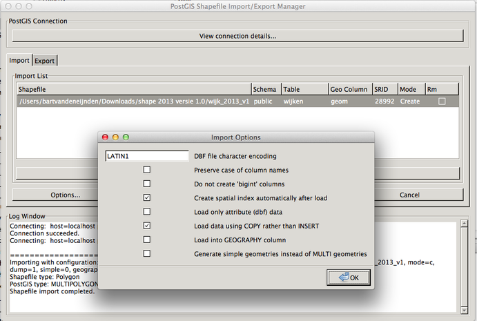
Note that, that the shapefile contains a number of attributes such as wk_naam.
Our challenge now is to set up a rendering system that can easily render any of our 59 columns of census data as a map.
We could define 59 layers in GeoServer, and set up 59 separate styles to provide attractive renderings of each variable. But that would be a lot of work, and we’re much too lazy to do that. What we want is a single layer that can be re-used to render any column of interest.
Using a parametric SQL view we can define a SQL-based layer definition that allows us to change the column of interest by substituting a variable when making a WMS map rendering call.
For example, this SQL definition will allow us to substitute any column we want into the map rendering chain:
SELECT wk_code, wk_naam, gm_code, gm_naam, water, %column% AS data
FROM wijken;
According to the documentation (see section 3 table 1) the NoData values of the Wijken en Buurten dataset are set to -99999997, -99999998 and -99999999. To make sure that these are correctly displayed , these values need to be set to NULL. Execute the following sql query on the database opengeo to do this:
DO $$
DECLARE
   col_names CURSOR FOR  SELECT column_name as cn, data_type as dt
      from information_schema.columns
      where table_name='wijken';
BEGIN

   FOR col_name_row IN col_names LOOP
      IF  col_name_row.cn not in ('wk_code','wk_naam','gm_code','gm_naam','water', 'geom' ) THEN
         RAISE NOTICE 'Updating column %', col_name_row.cn;
         EXECUTE format ('UPDATE wijken SET %I=null WHERE CAST(%I AS int) in
         (-99999997,-99999998,-99999999)', col_name_row.cn, col_name_row.cn);
      END IF;
   END LOOP;
END $$;
Viewing our data via a parametric SQL view doesn’t quite get us over the goal line though, because we still need to create a thematic style for the data, and the data in our 59 columns have vastly different ranges and distributions:
We need to somehow get all this different data onto one scale, preferably one that provides for easy visual comparisons between variables.
The answer is to use the average and standard deviation of the data to normalize it to a standard scale.

For example:
Let’s try it on our own census data.
SELECT Avg(AANT_INW), Stddev(AANT_INW) FROM wijken;

--           avg          |      stddev
-- -----------------------+-------------------
--  6342.9073724007561437 | 9864.171304604906

SELECT Avg((AANT_INW - 6342.9073724007561437) / 9864.171304604906),
       Stddev((AANT_INW - 6342.9073724007561437) / 9864.171304604906)
FROM wijken;

--     avg    | stddev
-- -----------+--------
--      ~0    |     ~1
So we can easily convert any of our data into a scale that centers on 0 and where one standard deviation equals one unit just by normalizing the data with the average and standard deviation!
Our new parametric SQL view will look like this:
-- Precompute the Avg and StdDev,
WITH stats AS (
  SELECT Avg(%column%) AS avg,
         Stddev(%column%) AS stddev
  FROM wijken
)
SELECT
  wijken.gm_naam,
  wijken.wk_naam,
  wijken.geom,
  %column% as data
  (%column% - avg)/stddev AS normalized_data
FROM stats,wijken
The query first calculates the overall statistics for the column, then applies those stats to the data in the table wijken, serving up a normalized view of the data.
With our data normalized, we are ready to create one style to rule them all!
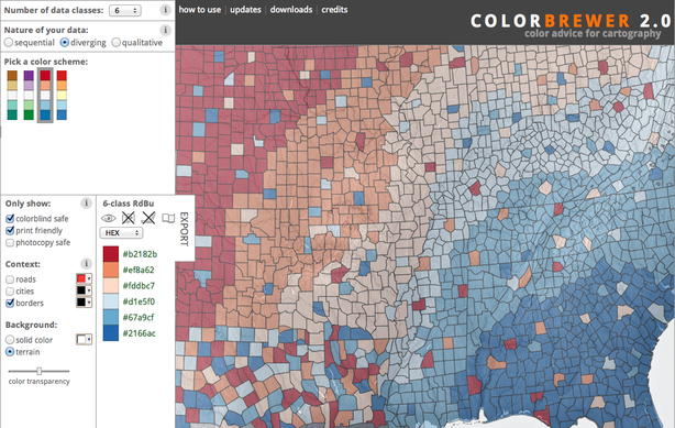
The colors above weren’t chosen randomly! We used ColorBrewer for creating this color scheme, because ColorBrewer provides palettes that have been tested for maximum readability and to some extent aesthetic quality. Here’s the palette for a bit of a Dutch atmosphere (although a red-blue color scale might not be the best option considering the normative assocation with these colors (blue good,red bad), a more neutral color scale could be a better option, feel free to experiment).
Note
You can access the OpenGeo Suite GeoServer through http://localhost:8080/geoserver/web/
Paste in the style definition (below) for stddev.xml and hit the Save button at the bottom
<NamedLayer>
  <Name>opengeo:stddev</Name>
  <UserStyle>

    <Name>Standard Deviation Ranges</Name>

    <FeatureTypeStyle>

      <Rule>
        <Name>StdDev < -1.0</Name>
        <ogc:Filter>
          <ogc:PropertyIsLessThan>
            <ogc:PropertyName>normalized_data</ogc:PropertyName>
            <ogc:Literal>-1.0</ogc:Literal>
          </ogc:PropertyIsLessThan>
        </ogc:Filter>
        <PolygonSymbolizer>
           <Fill>
              <!-- CssParameters allowed are fill and fill-opacity -->
              <CssParameter name="fill">#b2182b</CssParameter>
           </Fill>
           <Stroke>
             <CssParameter name="stroke">#1F1F1F</CssParameter>
             <CssParameter name="stroke-width">.25</CssParameter>
           </Stroke>
        </PolygonSymbolizer>
      </Rule>

      <Rule>
        <Name>-1.0 < StdDev < -0.5</Name>
        <ogc:Filter>
          <ogc:PropertyIsBetween>
            <ogc:PropertyName>normalized_data</ogc:PropertyName>
            <ogc:LowerBoundary>
              <ogc:Literal>-1.0</ogc:Literal>
            </ogc:LowerBoundary>
            <ogc:UpperBoundary>
              <ogc:Literal>-0.5</ogc:Literal>
            </ogc:UpperBoundary>
          </ogc:PropertyIsBetween>
        </ogc:Filter>
        <PolygonSymbolizer>
          <Fill>
            <!-- CssParameters allowed are fill and fill-opacity -->
            <CssParameter name="fill">#ef8a62</CssParameter>
          </Fill>
          <Stroke>
             <CssParameter name="stroke">#1F1F1F</CssParameter>
             <CssParameter name="stroke-width">.25</CssParameter>
           </Stroke>
        </PolygonSymbolizer>
      </Rule>

      <Rule>
        <Name>-0.5 < StdDev < 0.0</Name>
        <ogc:Filter>
          <ogc:PropertyIsBetween>
            <ogc:PropertyName>normalized_data</ogc:PropertyName>
            <ogc:LowerBoundary>
              <ogc:Literal>-0.5</ogc:Literal>
            </ogc:LowerBoundary>
            <ogc:UpperBoundary>
              <ogc:Literal>0.0</ogc:Literal>
            </ogc:UpperBoundary>
          </ogc:PropertyIsBetween>
        </ogc:Filter>
        <PolygonSymbolizer>
          <Fill>
            <!-- CssParameters allowed are fill and fill-opacity -->
            <CssParameter name="fill">#fddbc7</CssParameter>
          </Fill>
          <Stroke>
             <CssParameter name="stroke">#1F1F1F</CssParameter>
             <CssParameter name="stroke-width">.25</CssParameter>
           </Stroke>
        </PolygonSymbolizer>
      </Rule>

      <Rule>
        <Name>0.0 < StdDev < 0.5</Name>
        <ogc:Filter>
          <ogc:PropertyIsBetween>
            <ogc:PropertyName>normalized_data</ogc:PropertyName>
            <ogc:LowerBoundary>
              <ogc:Literal>0.0</ogc:Literal>
            </ogc:LowerBoundary>
            <ogc:UpperBoundary>
              <ogc:Literal>0.5</ogc:Literal>
            </ogc:UpperBoundary>
          </ogc:PropertyIsBetween>
        </ogc:Filter>
        <PolygonSymbolizer>
          <Fill>
            <!-- CssParameters allowed are fill and fill-opacity -->
            <CssParameter name="fill">#d1e5f0</CssParameter>
          </Fill>
          <Stroke>
             <CssParameter name="stroke">#1F1F1F</CssParameter>
             <CssParameter name="stroke-width">.25</CssParameter>
           </Stroke>
        </PolygonSymbolizer>
      </Rule>

      <Rule>
        <Name>0.5 < StdDev < 1.0</Name>
        <ogc:Filter>
          <ogc:PropertyIsBetween>
            <ogc:PropertyName>normalized_data</ogc:PropertyName>
            <ogc:LowerBoundary>
              <ogc:Literal>0.5</ogc:Literal>
            </ogc:LowerBoundary>
            <ogc:UpperBoundary>
              <ogc:Literal>1.0</ogc:Literal>
            </ogc:UpperBoundary>
          </ogc:PropertyIsBetween>
        </ogc:Filter>
        <PolygonSymbolizer>
          <Fill>
            <!-- CssParameters allowed are fill and fill-opacity -->
            <CssParameter name="fill">#67a9cf</CssParameter>
          </Fill>
          <Stroke>
             <CssParameter name="stroke">#1F1F1F</CssParameter>
             <CssParameter name="stroke-width">.25</CssParameter>
           </Stroke>
        </PolygonSymbolizer>
      </Rule>

      <Rule>
        <Name>1.0 < StdDev</Name>
        <ogc:Filter>
          <ogc:PropertyIsGreaterThan>
            <ogc:PropertyName>normalized_data</ogc:PropertyName>
            <ogc:Literal>1.0</ogc:Literal>
          </ogc:PropertyIsGreaterThan>
        </ogc:Filter>
        <PolygonSymbolizer>
           <Fill>
              <!-- CssParameters allowed are fill and fill-opacity -->
              <CssParameter name="fill">#2166ac</CssParameter>
           </Fill>
          <Stroke>
             <CssParameter name="stroke">#1F1F1F</CssParameter>
             <CssParameter name="stroke-width">.25</CssParameter>
           </Stroke>
        </PolygonSymbolizer>
      </Rule>

   </FeatureTypeStyle>
  </UserStyle>
</NamedLayer>
</StyledLayerDescriptor>
Now we have a style, we just need to create a layer that uses it!
First, we need a PostGIS store that connects to our database
You’ll be taken immediately to the New Layer panel (how handy) where you should:
-- Precompute the Avg and StdDev,
-- then normalize table
WITH stats AS (
SELECT Avg(%column%) AS avg,
       Stddev(%column%) AS stddev
FROM wijken
)
SELECT
wijken.geom,
wijken.wk_code as wijk_code,
wijken.wk_naam || 'Wijk' As wijk,
wijken.gm_naam || 'Gemeente' As gemeente,
'%column%'::text As variable,
%column%::real As data,
(%column% - avg)/stddev AS normalized_data
FROM stats, wijken
You’ll be taken immediately to the Edit Layer panel (how handy) where you should:
That’s it, the layer is ready!
We can change the column we’re viewing by altering the column view parameter in the WMS request URL.
The column names that the census uses are pretty opaque aren’t they? What we need is a web app that lets us see nice human readable column information, and also lets us change the column we’re viewing on the fly.
The first thing we need for our app is a data file that maps the short, unpractical column names in our census table to human readable information. Fortunately, the dictionary.txt file has all the information we need. The dictionary.txt file was created by copy pasting the text of the Buurten en Wijken documentation pdf in a text file and combining this with a list of all the columns of the Buurten en Wijken dataset with a python script.
The list of column names was necessary because the documentation of the Buurten en Wijken en dataset lists a lot more attributes than the file that we have downloaded from the NGR.
Here’s a couple example lines from the dictionary.txt file :
Each line has the column name and a human readable description. Fortunately the information is nicely seperated by a colon in the text file, so the fields can be extracted by using a split(":") function.
We’re going to consume this information in a JavaScript web application. The text file can easily be read in and split into lines. Each line can be split into an array with at position 0 the attribute code and at position 1 the attribute description to populate a topics dropdown.
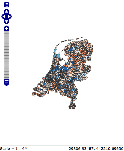
We already saw our map visualized in a bare OpenLayers 2 map frame in the Layer Preview section of GeoServer.
We want an application that provides a user interface component that manipulates the source WMS URL, altering the URL viewparams parameter.
We’ll build the app using Bootstrap for a straightforward layout with CSS, and OpenLayers 3 as the map component.
The base HTML page, index.html, contains script and stylesheet includes bringing in our various libraries. A custom stylesheet gives us a fullscreen map with a legend overlay. Bootstrap css classes are used to style the navigation bar. Containers for the map and a header navigation bar with the aforementioned topics dropdown are also included, and an image element with the legend image from a WMS GetLegendGraphic request is put inside the map container.
<!DOCTYPE html>
<html>
  <head>
    <title>Boundless Census Map</title>
    <!-- Bootstrap -->
    <link rel="stylesheet" href=
    "resources/bootstrap/css/bootstrap.min.css" type="text/css">
    <link rel="stylesheet" href=
    "resources/bootstrap/css/bootstrap-theme.min.css" type="text/css">
    <script src="resources/jquery-1.10.2.min.js"></script>
    <script src="resources/bootstrap/js/bootstrap.min.js"></script>
    <!-- OpenLayers -->
    <link rel="stylesheet" href="resources/ol3/ol.css">
    <script src="resources/ol3/ol.js"></script>
    <!-- Our Application -->
    <style>
      html, body, #map {
        height: 100%;
      }
      #map {
        padding-top: 50px;
      }
      .legend {
        position: absolute;
        z-index: 1;
        left: 10px;
        bottom: 10px;
        opacity: 0.6;
      }
    </style>
  </head>
  <body>
    <nav class="navbar navbar-inverse navbar-fixed-top"
    role="navigation">
      <div class="navbar-header">
        <a class="navbar-brand" href="#">Boundless Census Map</a>
      </div>
      <form class="navbar-form navbar-right">
        <div class="form-group">
          <select id="topics" class="form-control"></select>
        </div>
      </form>
    </nav>
    <div id="map">
      <!-- GetLegendGraphic, customized with some LEGEND_OPTIONS -->
      <img class="legend img-rounded" src=
       "https://workshop-boundless-geocat.geocat.net/geoserver/opengeo/wms?REQUEST=
       GetLegendGraphic&VERSION=1.3.0&FORMAT=image/png&WIDTH=26&HEIGHT=18&
       STRICT=false&LAYER=normalized&LEGEND_OPTIONS=fontName:sans-serif;
       fontSize:11;fontAntiAliasing:true;fontStyle:normal;fontColor:0xFFFFFF;
       bgColor:0x000000;">
    </div>
    <script type="text/javascript" src="wijkenkaart.js"></script>
  </body>
</html>
The real code is in the wijkenkaart.js file. We start by creating an Openbasiskaart base layer, and adding our parameterized census layer on top as an image layer with a WMS Layer source.
// Base map
var extent = [-285401.920000,22598.080000,595401.920000,903401.920000];
var resolutions = [3440.64,1720.32,860.16,430.08,215.04,107.52,53.76,26.88,
13.44,6.72,3.36,1.68,0.84,0.42,0.21];

var projection = new ol.proj.Projection({
    code: 'EPSG:28992',
    units: 'meters',
    extent: extent
});

var url = 'http://openbasiskaart.nl/mapcache/tms/1.0.0/osm@rd/';

var tileUrlFunction = function(tileCoord, pixelRatio, projection) {
  var zxy = tileCoord;
  if (zxy[1] < 0 || zxy[2] < 0) {
    return "";
  }
  return url +
    zxy[0].toString()+'/'+ zxy[1].toString() +'/'+
    zxy[2].toString() +'.png';
};

var openbasiskaartLayer = new ol.layer.Tile({
  preload: 0,
  source: new ol.source.TileImage({
    crossOrigin: null,
    extent: extent,
    projection: projection,
    tileGrid: new ol.tilegrid.TileGrid({
      origin: [-285401.920000,22598.080000],
      resolutions: resolutions
    }),
    tileUrlFunction: tileUrlFunction
  })
});

// Census map layer
var wmsLayer = new ol.layer.Image({
  source: new ol.source.ImageWMS({
    url: 'https://workshop-boundless-geocat.geocat.net/geoserver/opengeo/wms?',
    params: {'LAYERS': 'normalized'}
  }),
  opacity: 0.6
});

// Map object
olMap = new ol.Map({
  target: 'map',
  layers: [
  openbasiskaartLayer, wmsLayer
  ],
  view: new ol.View({
    projection: projection,
    center: [150000, 450000],
    zoom: 2
  })
});
We configure an OpenLayers Map, assign the layers, and give it a map view with a center and zoom level. Now the map will load.
The select element with the id topics will be our drop-down list of available columns. We load the dictionary.txt file, and fill the select element with its contents. This is done by adding an option child for each line.
// Load variables into dropdown
$.get("../data/dictionary.txt", function(response) {
  // We start at line 3 - line 1 is column names, line 2 is not a variable
  $(response.split('\n')).each(function(index, line) {
    $('#topics').append($("<option>")
      .val(line.split(":")[0].trim())
      .html(line.split(":")[1].trim()));
  });
});

// Add behaviour to dropdown
$('#topics').change(function() {
  wmsLayer.getSource().updateParams({
    'viewparams': 'column:' + $('#topics>option:selected').val()
  });
});
Look at the the wijkenkaart.js file to see the whole application in one page.
When we open the index.html file, we see the application in action.
We’ve built an application for browsing 59 different census variables, using less than 100 lines of JavaScript application code, and demonstrating:
Try to implement one of these examples in your own map.
Workshop created for GeoBuzz 2014 by GeoCat and Boundless. Workshop heavily inspired/copied from Building a Census Map.
Workshop licensed under Creative Commons by-nc-sa.
Contact: Anton Bakker and Bart van den Eijnden.